作业6 线性 岭回归 多项式

README.md

@@ -2,3 +2,9 @@
 
 课程作业
 
+
+## eda
+
+演示地址
+
+https://edaf.veypi.com

numerical_analysis/1/README.md

@@ -56,5 +56,8 @@ end
 作业提交有效时间是今天到10月23日（两周后）之前的任意时间。提交作业请将代码和报告打包，以“课后作业1-名字-学号”命名提交。
 
 
+![image-20210116232529898](https://public.veypi.com/img/screenshot/20210116232529.png)
 
+![image-20210116235118221](https://public.veypi.com/img/screenshot/20210116235118.png)
 
+![image-20210116235324496](https://public.veypi.com/img/screenshot/20210116235324.png)

numerical_analysis/1/main.py

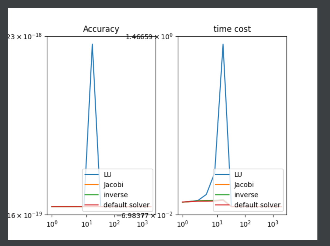
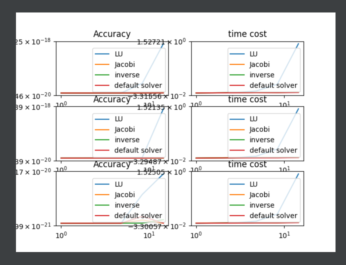
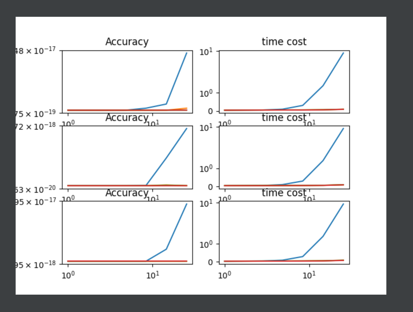
@@ -0,0 +1,184 @@
+import numpy as np
+import matplotlib.pyplot as plt
+import time
+
+
+def LU_decomposition(A):
+    n = len(A[0])
+    L = np.zeros([n, n])
+    U = np.zeros([n, n])
+    for i in range(n):
+        L[i][i] = 1
+        if i == 0:
+            U[0][0] = A[0][0]
+            for j in range(1, n):
+                U[0][j] = A[0][j]
+                L[j][0] = A[j][0] / U[0][0]
+        else:
+            for j in range(i, n):  # U
+                temp = 0
+                for k in range(0, i):
+                    temp = temp + L[i][k] * U[k][j]
+                U[i][j] = A[i][j] - temp
+            for j in range(i + 1, n):  # L
+                temp = 0
+                for k in range(0, i):
+                    temp = temp + L[j][k] * U[k][i]
+                L[j][i] = (A[j][i] - temp) / U[i][i]
+    return L, U
+
+
+# 生成随机矩阵 A, b, 范围[-10, 10]
+def randomAb(m):
+    A = np.random.random([m, m]) * 20 - 10
+    dia = np.random.random(m) * 10
+    for i in range(len(dia)):
+        A[i, i] = dia[i]
+    return A, np.random.randint(0, 10, [m, 1])
+
+
+# 生成稀疏矩阵A, b
+def sparseMatrix(m):
+    A, b = randomAb(m)
+    for i in range(m):
+        for j in range(m):
+            if i != j:
+                a = A[i][j]
+                if abs(a) < 9:
+                    A[i][j] = 0
+                elif a > 0:
+                    A[i][j] = 10 * (a - 9)
+                else:
+                    A[i][j] = 10 * (9 + a)
+
+    return A, b
+
+
+# 生成病态矩阵A, b
+def illMatrix(m):
+    A, b = randomAb(m)
+    return A, b
+
+
+class Question1:
+    """
+    求解 Ax=b
+    """
+
+    def __init__(self):
+        pass
+
+    def solver1(self, A, b):
+        """
+        LU 分解 求解器
+        """
+        L, U = LU_decomposition(A)
+        # LY=b
+        n = len(A)
+        y = np.zeros((n, 1))
+        for i in range(len(A)):
+            t = 0
+            for j in range(i):
+                t += L[i][j] * y[j][0]
+            y[i][0] = b[i][0] - t
+        X = np.zeros((n, 1))
+        for i in range(len(A) - 1, -1, -1):
+            t = 0
+            for j in range(i + 1, len(A)):
+                t += U[i][j] * X[j][0]
+            t = y[i][0] - t
+            if t != 0 and U[i][i] == 0:
+                return 0
+            X[i] = t / U[i][i]
+        return X
+
+    def solver2(self, A, b):
+        """
+        Jacobi 求解器
+        """
+        x = np.zeros(b.shape)
+        Dv = np.diag(A)
+        D = np.zeros(A.shape)
+        for i in range(len(Dv)):
+            D[i, i] = Dv[i]
+        R = A - np.diagflat(Dv)
+
+        # Iterate for N times
+        print(D)
+        D = np.linalg.inv(D)
+        print(D)
+        while 1:
+            x1 = D @ (b - R @ x)
+            if np.max(x1 - x) < 1e-6:
+                break
+            x = x1
+        return x
+        # return Jacobi(np.zeros(b.shape), A, b)
+
+    def solver3(self, A, b):
+        """
+        inv(A) * b
+        """
+        return np.dot(np.linalg.inv(A), b)
+
+    def solver4(self, A, b):
+        """
+        默认求解器
+        """
+        return np.linalg.solve(A, b)
+
+    def RMSE(self, solver, n=8, randFunc=randomAb):
+        ## 计算方差
+        s = time.time()
+        A, b = randFunc(n)
+        X = (A.dot(solver(A, b)) - b) ** 2
+        for i in range(1000):
+            A, b = randFunc(n)
+            X = X + (A.dot(solver(A, b)) - b) ** 2
+        return np.max(X), time.time() - s
+
+    def show(self):
+        n = 12
+        N = [2 ** i for i in range(n)]
+        Y = [[0 for i in range(n)] for _ in range(4)]
+        Z = [[0 for i in range(n)] for _ in range(4)]
+
+        randomFuns = [randomAb, sparseMatrix, illMatrix]
+        for r in range(3):
+            plt.subplot(3, 2, 2*r + 1)
+            for i in range(n):
+                print("size: %s" % N[i])
+                print("LU")
+                Y[0][i], Z[0][i] = self.RMSE(self.solver1, N[i])
+                print("jacobi")
+                Y[1][i], Z[1][i] = self.RMSE(self.solver3, N[i])
+                print("inverse")
+                Y[2][i], Z[2][i] = self.RMSE(self.solver3, N[i])
+                print("default\n")
+                Y[3][i], Z[3][i] = self.RMSE(self.solver4, N[i])
+
+            # N = range(12)
+            plt.plot(N, Y[0], label="LU")
+            plt.plot(N, Y[1], label="Jacobi")
+            plt.plot(N, Y[2], label="inverse")
+            plt.plot(N, Y[3], label="default solver")
+            # plt.xticks([0, 10, 100, 1000], [0, 10, 100, 1000])
+            plt.title('Accuracy')
+            plt.yscale('symlog')
+            plt.xscale('symlog')
+            # plt.legend(loc='lower right')
+            plt.subplot(3, 2, 2 * r + 2)
+            plt.plot(N, Z[0], label="LU")
+            plt.plot(N, Z[1], label="Jacobi")
+            plt.plot(N, Z[2], label="inverse")
+            plt.plot(N, Z[3], label="default solver")
+            plt.xscale('symlog')
+            plt.yscale('symlog')
+            plt.title('time cost')
+            # plt.legend(loc='lower right')
+        plt.show()
+
+
+if __name__ == "__main__":
+    q = Question1()
+    q.show()

numerical_analysis/2/README.md

@@ -0,0 +1,17 @@
+# 结论
+
+图例
+
+    0 - 标准函数
+    1 - 复化梯形公式
+    2 -  复化Simpson 1/3
+    3 -  复化Simpson 3/8
+
+随积分区间变化图
+
+![image-20210117003720172](https://public.veypi.com/img/screenshot/20210117003720.png)
+
+
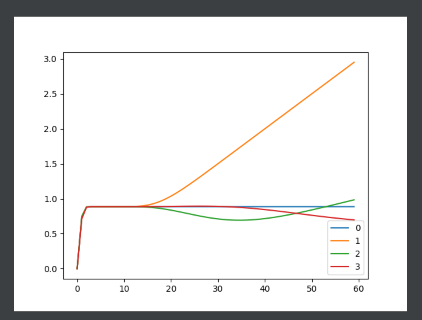
+随N变化图
+
+![image-20210117004402891](https://public.veypi.com/img/screenshot/20210117004402.png)

numerical_analysis/2/main.py

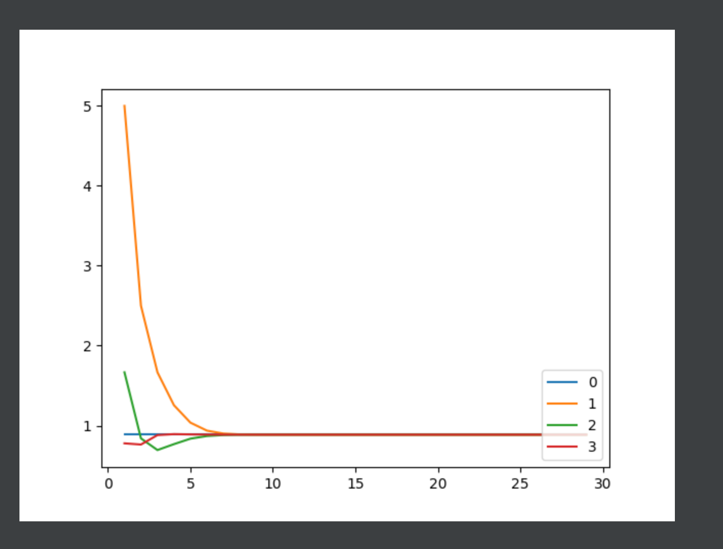
@@ -0,0 +1,90 @@
+import math
+from scipy import integrate
+import matplotlib.pyplot as plt
+
+
+def erf_inner(x):
+    return math.e ** (- x ** 2)
+
+
+def solve0(a, b, N):
+    """
+    标准函数求积分
+    """
+    return integrate.quad(erf_inner, a, b)[0]
+
+
+def solve1(a, b, N):
+    """
+    复化梯形积分公式
+    """
+    h = (b - a) / N
+    s = erf_inner(a)
+    for i in range(1, N):
+        s += 2 * erf_inner(a + h * i)
+    s += erf_inner(b)
+    return s * h / 2
+
+
+def solve2(a, b, N):
+    """
+    复化Simpson 1/3
+    """
+    h = (b - a) / N
+    s = 0
+    s = erf_inner(a)
+    for i in range(1, N):
+        s += 2 * erf_inner(a + h * i)
+    for i in range(0, N):
+        s += 4 * erf_inner(a + h * (i + 0.5))
+    s += erf_inner(b)
+    return s * h / 6
+
+
+def solve3(a, b, N):
+    """
+    复化Simpson 3/8
+    """
+    h = (b - a) / N
+    s = 0
+    s = 7 * erf_inner(a)
+    for i in range(1, N):
+        s += 32 * erf_inner(a + h * (i - 0.75)) + 12 * erf_inner(a + h * (i - 0.5)) + 32 * erf_inner(
+            a + h * (i - 0.25)) + 14 * erf_inner(a + h * i)
+    s += 7 * erf_inner(b)
+    return s * h / 90
+
+
+def show():
+    x = [i for i in range(60)]
+    y = [[0 for j in range(60)] for _ in range(4)]
+    solves = [solve0, solve1, solve2, solve3]
+    for s in range(4):
+        for i in x:
+            y[s][i] = solves[s](0, i, 10)
+        plt.plot(x, y[s], label=str(s))
+    plt.legend(loc="lower right")
+    plt.show()
+
+
+def showN():
+    x = [i for i in range(1, 30)]
+    y = [[0 for j in range(30)] for _ in range(4)]
+    solves = [solve0, solve1, solve2, solve3]
+    for s in range(4):
+        for i in x:
+            y[s][i] = solves[s](0, 10, i)
+        plt.plot(x, y[s][1:], label=str(s))
+    plt.legend(loc="lower right")
+    plt.show()
+
+
+if __name__ == '__main__':
+    # a = 0
+    # b = 20
+    # n = 90
+    # print(solve1(a, b, n))
+    # print(solve2(a, b, n))
+    # print(solve3(a, b, n))
+    # print(solve0(a, b, n))
+    showN()

numerical_analysis/3/README.md

@@ -0,0 +1,18 @@
+
+# 问题1
+
+1:
+    f = 1 / (e^(-x) + e^x)
+
+2
+
+标签
+
+    0： 默认求解器
+    1： 向前差分
+    2： 向后差分
+    3： rk45
+
+![image-20210117035636815](https://public.veypi.com/img/screenshot/20210117035636.png)
+
+![image-20210117040727886](https://public.veypi.com/img/screenshot/20210117040727.png)

numerical_analysis/3/main.py

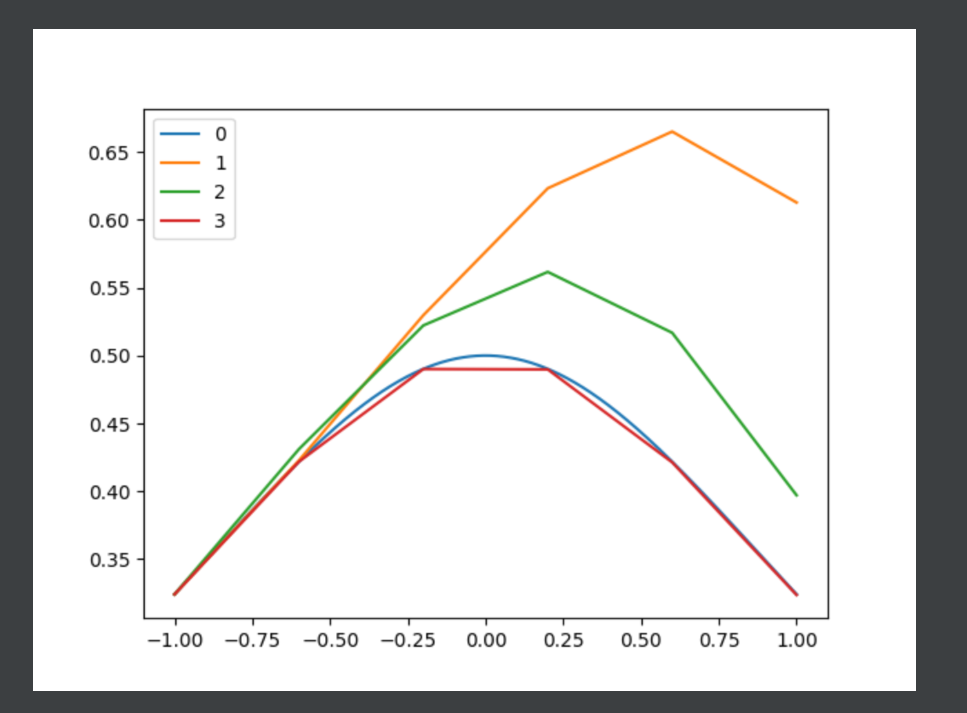
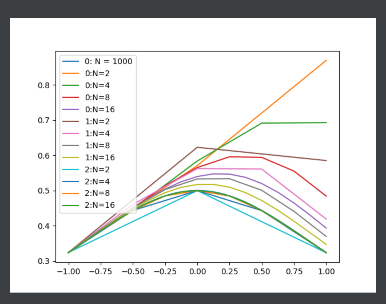
@@ -0,0 +1,153 @@
+import math
+from math import e
+import numpy as np
+import matplotlib.pyplot as plt
+from scipy.integrate import odeint, solve_bvp, solve_ivp
+
+
+def runge_kutta(y, x, dx, f):
+    """ y is the initial value for y
+        x is the initial value for x
+        dx is the time step in x
+        f is derivative of function y(t)
+    """
+    k1 = dx * f(y, x)
+    k2 = dx * f(y + 0.5 * k1, x + 0.5 * dx)
+    k3 = dx * f(y + 0.5 * k2, x + 0.5 * dx)
+    k4 = dx * f(y + k3, x + dx)
+    return y + (k1 + 2 * k2 + 2 * k3 + k4) / 6.
+
+
+'''
+    为了兼容solve_ivp的参数形式，微分方程函数定义的参数顺序为(t,y)，因此使用odeint函数时需要使参数tfirst=True
+    二阶甚至高阶微分方程组都可以变量替换成一阶方程组的形式，再调用相关函数进行求解，因此编写函数的时候，不同于一阶微分方程，二阶或者高阶微分方程返回的是低阶到高阶组成的方程组，
+
+'''
+
+y0 = [1 / (e + 1 / e), (e - 1 / e) / ((e + 1 / e) ** 2)]  # 初值条件
+
+
+# 初值[2,0]表示y(0)=2,y'(0)=0
+
+
+def fvdp1(t, y):
+    '''
+    要把y看出一个向量，y = [dy0,dy1,dy2,...]分别表示y的n阶导，那么
+    y[0]就是需要求解的函数，y[1]表示一阶导，y[2]表示二阶导，以此类推
+    对于二阶微分方程，肯定是由0阶和1阶函数组合而成的，所以下面把y看成向量的话，y0表示最初始的函数，也就是我们要求解的函数，y1表示一阶导，对于高阶微分方程也可以以此类推
+    '''
+    dy1 = y[1]  # y[1]=dy/dt，一阶导
+    # dy2 = -3 * y[1] - 2 * y[0] + np.exp(-1 * t)
+    dy2 = 2 * y[1] ** 2 / y[0] - y[0]
+    # y[0]是最初始，也就是需要求解的函数
+    # 注意返回的顺序是[一阶导， 二阶导]，这就形成了一阶微分方程组
+    return [dy1, dy2]
+
+
+def solve0():
+    '''
+    内置求解器1
+    '''
+    t2 = np.linspace(-1, 1, 1000)
+    return odeint(fvdp1, y0, t2, tfirst=True)[:, 0]
+
+
+def solve01(seq):
+    f0 = [y0[0]]
+    f1 = [y0[1]]
+    f2 = [fvdp1(-1, [f0[0], f1[0]])[1]]
+    for i in range(1, len(seq)):
+        h = seq[i] - seq[i - 1]
+        k21 = f2[i - 1]
+        k22 = fvdp1(seq[i - 1] + h / 2, [f0[i - 1] + h * k21 / 2, f1[i - 1] + h * k21 / 2])[1]
+        k23 = fvdp1(seq[i - 1] + h / 2, [f0[i - 1] + h * k22 / 2, f1[i - 1] + h * k22 / 2])[1]
+        k24 = fvdp1(seq[i - 1] + h / 2, [f0[i - 1] + h * k23, f1[i - 1] + h * k23])[1]
+        f1.append(f1[i - 1] + h * (k21 + k22 + k23 + k24) / 6)
+        f0.append(f0[i - 1] + h * f1[i - 1])
+        f2.append(fvdp1(seq[i], [f0[i], f1[i]])[1])
+    return f0
+
+
+def solve1(seq):
+    '''
+    向前差分
+    '''
+    f0 = [y0[0]]
+    f1 = [y0[1]]
+    f2 = [fvdp1(-1, [f0[0], f1[0]])[1]]
+    for i in range(1, len(seq)):
+        h = seq[i] - seq[i - 1]
+        f0.append(f0[i - 1] + h * f1[i - 1])
+        f1.append(f1[i - 1] + h * f2[i - 1])
+        f2.append(fvdp1(seq[i], [f0[i], f1[i]])[1])
+    return f0
+
+
+def solve2(seq):
+    '''
+    向后差分
+    '''
+    f0 = [y0[0]]
+    f1 = [y0[1]]
+    f2 = [fvdp1(-1, [f0[0], f1[0]])[1]]
+    for i in range(1, len(seq)):
+        h = seq[i] - seq[i - 1]
+        f2.append(fvdp1(seq[i], [f0[i - 1], f1[i - 1]])[1])
+        f1.append(f1[i - 1] + h * f2[i])
+        f0.append(f0[i - 1] + h * f1[i])
+    return f0
+
+
+def runge_kutta(y, x, dx, f):
+    """ y is the initial value for y
+        x is the initial value for x
+        dx is the time step in x
+        f is derivative of function y(t)
+    """
+    k1 = dx * f(y, x)
+    k2 = dx * f(y + 0.5 * k1, x + 0.5 * dx)
+    k3 = dx * f(y + 0.5 * k2, x + 0.5 * dx)
+    k4 = dx * f(y + k3, x + dx)
+    return y + (k1 + 2 * k2 + 2 * k3 + k4) / 6.
+
+
+def solve3(seq):
+    '''
+    rk4
+    '''
+    return solve_ivp(fvdp1, t_span=(-1, 1.0), y0=y0, t_eval=seq).y.T[:, 0]
+
+
+def show():
+    t0 = np.linspace(-1, 1, 1000)
+    r0 = solve0()
+    t1 = np.linspace(-1, 1, 6)
+    r1 = solve1(t1)
+    t2 = np.linspace(-1, 1, 6)
+    r2 = solve2(t2)
+    t3 = np.linspace(-1, 1, 6)
+    r3 = solve3(t3)
+    plt.plot(t0, r0, label='0')
+    plt.plot(t1, r1, label='1')
+    plt.plot(t2, r2, label='2')
+    plt.plot(t3, r3, label='3')
+    plt.legend()
+    plt.show()
+
+
+def showN():
+    t0 = np.linspace(-1, 1, 1000)
+    r0 = solve0()
+    plt.plot(t0, r0, label='0: N = 1000')
+    solves = [solve1, solve2, solve3]
+    for j in range(3):
+        for i in range(1, 5):
+            n = 2 ** i
+            t = np.linspace(-1, 1, n + 1)
+            plt.plot(t, solves[j](t), label='%s:N=%s' % (j, n))
+    plt.legend()
+    plt.show()
+
+
+if __name__ == '__main__':
+    showN()

numerical_analysis/5/README.md

@@ -0,0 +1,5 @@
+![image-20210117042146956](https://public.veypi.com/img/screenshot/20210117042146.png)
+
+![image-20210117043700038](https://public.veypi.com/img/screenshot/20210117043700.png)
+
+![image-20210117043750115](https://public.veypi.com/img/screenshot/20210117043750.png)

numerical_analysis/5/main.py

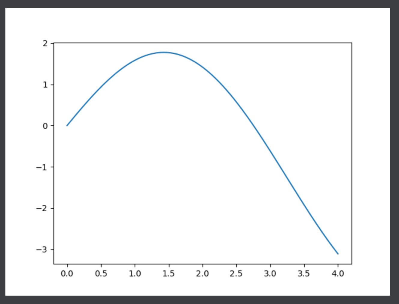
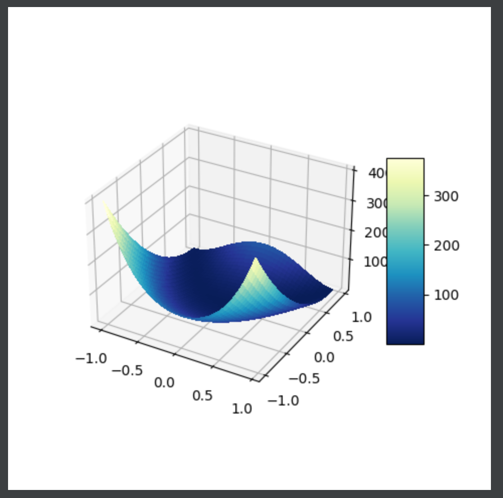
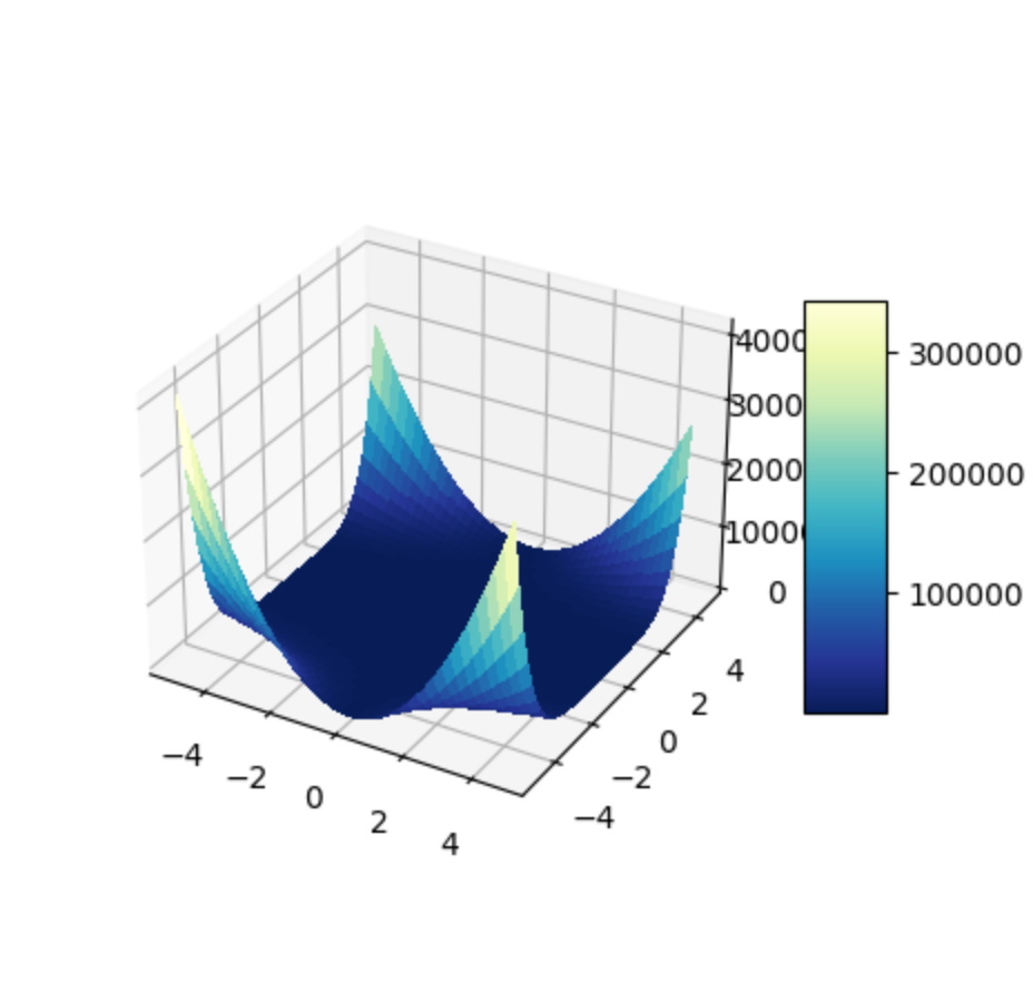
@@ -0,0 +1,60 @@
+import math
+import matplotlib.pyplot as plt
+import numpy as np
+from matplotlib.ticker import LinearLocator
+
+
+def f1(x):
+    return 2 * math.sin(x) - x ** 2 / 10
+
+
+def showf1():
+    t = np.linspace(0, 4, 1000)
+    plt.plot(t, [f1(x) for x in t])
+    plt.show()
+
+
+def f2(x, y):
+    return (1 - x) ** 2 + 100 * (y - x ** 2) ** 2
+
+
+def f3(x, y):
+    return (1.5 - x + x * y) ** 2 + (2.25 - x + x * y ** 2) ** 2 + (2.625 - x + x * y ** 3) ** 2
+
+
+def showf2():
+    fig = plt.figure(figsize=plt.figaspect(1.))
+    ax = fig.add_subplot(1, 1, 1, projection='3d')
+    X = np.arange(-1, 1, 0.05)
+    Y = np.arange(-1, 1, 0.05)
+    X, Y = np.meshgrid(X, Y)
+    # R = np.sqrt(X ** 2 + Y ** 2)
+    Z = f2(X, Y)
+    # Z = np.sin(R)
+
+    surf = ax.plot_surface(X, Y, Z, rstride=1, cstride=1,
+                           cmap=plt.cm.YlGnBu_r,
+                           linewidth=0, antialiased=False)
+    fig.colorbar(surf, shrink=0.5, aspect=5)
+    plt.show()
+
+
+def showf3():
+    fig = plt.figure(figsize=plt.figaspect(1.))
+    ax = fig.add_subplot(1, 1, 1, projection='3d')
+    X = np.arange(-5, 5, 0.25)
+    Y = np.arange(-5, 5, 0.25)
+    X, Y = np.meshgrid(X, Y)
+    # R = np.sqrt(X ** 2 + Y ** 2)
+    Z = f3(X, Y)
+    # Z = np.sin(R)
+
+    surf = ax.plot_surface(X, Y, Z, rstride=1, cstride=1,
+                           cmap=plt.cm.YlGnBu_r,
+                           linewidth=0, antialiased=False)
+    fig.colorbar(surf, shrink=0.5, aspect=5)
+    plt.show()
+
+
+if __name__ == '__main__':
+    showf3()

numerical_analysis/6/README.md

@@ -0,0 +1,2 @@
+
+![image-20210117045857685](https://public.veypi.com/img/screenshot/20210117045857.png)

numerical_analysis/6/main.py

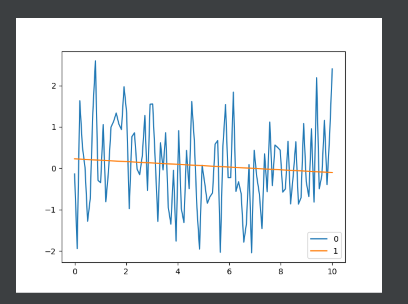
@@ -0,0 +1,46 @@
+import math
+import matplotlib.pyplot as plt
+import numpy as np
+import random
+from sklearn.linear_model import LinearRegression, Ridge, RidgeCV
+from sklearn.preprocessing import PolynomialFeatures
+
+
+def f1(x, e):
+    return math.exp(-x) * math.sin(x) \
+           + random.normalvariate(0, e)
+
+
+def f2(x, y, e):
+    return math.exp(-x ** 2 - y ** 2) * math.sin(x * y) + random.normalvariate(0, e)
+
+
+def solve1(x, y):
+    return LinearRegression().fit(x, y)
+
+
+def solve2(x, y):
+    poly = PolynomialFeatures(degree=4)
+    X_poly = poly.fit_transform(x)
+    poly.fit(X_poly, y)
+    return poly
+
+
+def solve3(x, y):
+    model = RidgeCV(alphas=[0.1, 1.0, 10.0])  # 通过RidgeCV可以设置多个参数值，算法使用交叉验证获取最佳参数值
+    model.fit(x, y)
+    return model
+
+
+if __name__ == '__main__':
+    x = np.linspace(0, 10, 100)
+    data = [f1(i, 1) for i in x]
+    y1 = []
+    model = solve3(x.reshape((-1, 1)), data)
+    for i in x:
+        y1.append(model.predict([[i]])[0])
+    print(model.predict([[1]]))
+    plt.plot(x, data, label='0')
+    plt.plot(x, y1, label='1')
+    plt.legend()
+    plt.show()

numerical_analysis/8/main.py

@@ -108,6 +108,6 @@ class WinePredict:
 if __name__ == '__main__':
     wp = WinePredict()
     wp.gs_rfc()
-    for i in [wp.rfc, wp.lr, wp.svc, wp.sgd, wp.mlp][:1]:
+    for i in [wp.rfc, wp.lr, wp.svc, wp.sgd, wp.mlp]:
         wp.report(i)
     # wp.showXY()